Monthly Algorithmic Challenge (September 2023): Sum of Two Numbers

---

Problem

This post is the third in the sequence of monthly mechanistic interpretability challenges. I designed them in the spirit of Stephen Casper's challenges, but with the more specific aim of working well in the context of the rest of the ARENA material, and helping people put into practice all the things they've learned so far. You can access the full ARENA materials from the Streamlit page. The purpose of the page you're currently reading is mainly to provide an easy-to-access place to read the solutions and understand the nature of these problems; I'd recommend using the Streamlit page instead if you're actually working through the problems. You can also find the solutions Colab here. I'll assume everyone has read the first problem, and has some overall context on the sequence.

Task & Dataset

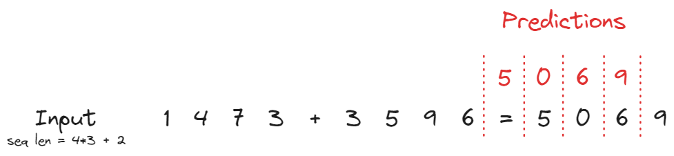
The problem for this month is interpreting a model which has been trained to perform simple addition. The model was fed input in the form of a sequence of digits (plus special + and = characters with token ids 10 and 11), and was tasked with predicting the sum of digits one sequence position before they would appear. Cross entropy loss was only applied to these four token positions, so the model's output at other sequence positions is meaningless.

All the left-hand numbers are below 5000, so we don't have to worry about carrying past the thousands digit.

Here is an example of what this dataset looks like:

dataset = SumDataset(size=1, num_digits=4, seed=42)

print(dataset[0].tolist()) # tokens, for passing into model
print("".join(dataset.str_toks[0])) # string tokens, for printing

Model

Our model was trained by minimising cross-entropy loss between its predictions and the true labels, at the four positions of the sum's digits. You can inspect the notebook training_model.ipynb to see how it was trained. I used the version of the model which achieved highest accuracy over 50 epochs (accuracy ~99%).

The model is is a 2-layer transformer with 2 attention heads, and causal attention. It includes layernorm, but no MLP layers.

Solutions

First, let's do some setup:

dataset = SumDataset(size=1000, num_digits=4, seed=42).to(device)
N = len(dataset)

# Define some useful objects
LABELS_STR = ['A0', 'A1', 'A2', 'A3', '+', 'B0', 'B1', 'B2', 'B3', '=', 'C0', 'C1', 'C2', 'C3']
LABELS_HTML = [f"A{i}" for i in range(4)] + ["+"] + [f"B{i}" for i in range(4)] + ["="] + [f"C{i}" for i in range(4)]
LABELS_DICT = {label: i for i, label in enumerate(LABELS_STR)}

targets = dataset.toks[:, -4:]

logits, cache = model.run_with_cache(dataset.toks)
logits: Tensor = logits[:, -5:-1]

logprobs = logits.log_softmax(-1) # [batch seq_len vocab_out]
probs = logprobs.softmax(-1)

batch_size, seq_len = dataset.toks.shape
logprobs_correct = eindex(logprobs, targets, "batch seq [batch seq]")
probs_correct = eindex(probs, targets, "batch seq [batch seq]")

avg_cross_entropy_loss = -logprobs_correct.mean().item()

print(f"Average cross entropy loss: {avg_cross_entropy_loss:.3f}")
print(f"Mean probability on correct label: {probs_correct.mean():.3f}")
print(f"Median probability on correct label: {probs_correct.median():.3f}")
print(f"Min probability on correct label: {probs_correct.min():.3f}")

And some simple (kinda hacky) visualisation:

def show(i):

    imshow(
        probs[i].T,
        y=dataset.vocab,
        x=[f"{dataset.str_toks[i][j]}<br><sub>({j})</sub>" for j in range(9, 13)],
        labels={"x": "Token", "y": "Vocab"},
        xaxis_tickangle=0,
        title=f"Sample model probabilities:<br>{''.join(dataset.str_toks[i])}",
        text=[
            ["〇" if (str_tok == target) else "" for target in dataset.str_toks[i][-4:]]
            for str_tok in dataset.vocab
        ],
        width=400,
        height=550,
    )

show(0)

Summary of how the model works

Let's start at the end - how the model actually represents each digit, as a prediction.

By the end of layer 1, the residual stream is parameterized by a single value: the angle $\theta$. The digits from 0-9 are evenly spaced around the unit circle, and the model's prediction depends on which angle they're closest to (the span of the unembedding matrix is basically the same as the span of these two vectors). Two visualisations of this are shown below: (1) the singular value decomposition of the unembedding matrix, and (2) the residual stream projected onto these first two singular directions.

So this is how the model predicts a digit at the end - how does it get those predictions in the first place?

To calculate each digit Ci, we require 2 components - the sum and the carry. The formula for Ci is (sum + int(carry == True)) % 10, where sum is the sum of digits Ai + Bi, and carry is whether A(i+1) + B(i+1) >= 10. (This ignores issues of carrying digits multiple times, which I won't discuss in this solution.)

We calculate the carry by using the hierarchy $0 > 9 > 1 > 8 > ... > 4 > 5$. An attention head in layer 0 will attend to the first number in this hierarchy that it sees, and if that number is $\geq 5$ then that means the digit will be carried. There are also some layer 0 attention heads which store the sum information in certain sequence positions - either by attending uniformly to both digits, or by following the reverse hierarchy so it can additively combine with something that follows the hierarchy. Below is a visualisation of the QK circuits for the layer 0 attention heads at the positions which are storing this "carry" information, to show how they're implementing the hierarchy:

At the end of layer 0, the "sum information" is stored in the residual stream as points around a circle traced out by two vectors, parameterized by an angle $\theta$. The "carry information" is stored in the residual stream as a single direction.

The model manages to store the sum of the two digits modulo 10 in a circular way by the end of layer 0 (although it's not stored in exactly the same way it will be at the end of the model). We might guess the model takes advantage of some trig identities to do this, although I didn't have time to verify this conclusively.

The heads in layer 1 mostly process this information by self-attending. They seem to be mostly clearing up some of the representations learned by the layer 0 heads, and implementing the "carrying digits" logic (since carrying a digit is equivalent to a rotation of $\pi/5$ around the circle, in the second figure above).

Notation

We'll refer to the sequence positions as A0, A1, A2, A3, +, B0, B1, B2, B3, =, C0, C1, C2, C3.

Usually, this will refer to those sequence positions, but sometimes it'll refer to the tokens at those sequence positions (hopefully it'll be clear which one we mean from context).

Some initial notes

• There are 2 different parts of figuring out each digit: adding two things together, and figuring out whether the digit needs to be incremented
• I expect the problem to be easiest when looking at the units digit, because there's no incrementation to worry about
• I expect all other digits to be implementing something of the form "do the units digit alg, plus do other things to compute whether a digit needs to be carried"
• To make life simpler, I could create a dataset which only contains digits that don't require any carrying (e.g. all digits were uniform between 0 and 4 inclusive)

Things I expect to see:

• Attention patterns
  1. There will be a head / heads in layer 0, which attend from X back to the two digits that are being added together to create X
  2. There will be a head / heads in layer 1, which have a more difficult job: figuring out incrementation
• Full matrices: QK
  1. The layer 0 head mentioned above will have a QK circuit that is only a function of position (it'll deliberately ignore token information cause it needs to always get an even split)
• Other things
  • Neel's modular arithmetic model used Fourier stuff to implement modular arithmetic. I'm essentially doing modular arithmetic here too, since I'm calculating the sum of 2 digits modulo 10. It's possible this is just done via some memorization system (cause it's a much smaller dataset than Neel's model was trained with), but I'd weakly guess Fourier stuff is involved.

First pass - attention patterns, and ablations

First experiments - we'll look at the attention patterns, then narrow in on the heads which are doing the thing we think must happen (i.e. equal attention back to both digits). Do we see what we expect to see?

Before doing attention patterns though, I'll plot the mean attention paid from to/from each combination of tokens. I'm expecting to see some patterns where the avg attention is approximately 0.5 for each of a pair of digits from the numbers being added together (because addition is a symmetric operation). We might guess that sequence positions in heads in layer 0 which don't have this "uniform average" aren't actually doing important things.

attn = t.concat([cache["pattern", layer] for layer in range(model.cfg.n_layers)], dim=1) # [batch heads seqQ seqK]

    imshow(
        attn.mean(0),
        facet_col=0,
        facet_labels=[f"{layer}.{head}" for layer in range(model.cfg.n_layers) for head in range(model.cfg.n_heads)],
        facet_col_wrap=model.cfg.n_heads,
        height=700,
        width=900,
        x=LABELS_STR,
        y=LABELS_STR,
    )

We can see a few positions in layer 0 which are paying close to 0.5 average attention to each of some two digits being added together (e.g. positions = and C0 in head 0.2). We don't see any patterns like this in layer 1.

Now, let's inspect attention patterns in actual examples.

cv.attention.from_cache(
    cache = cache,
    tokens = dataset.str_toks,
    batch_idx = list(range(10)),
    radioitems = True,
    return_mode = "view",
    batch_labels = ["".join(s) for s in dataset.str_toks],
    mode = "small",
)

Before we start over-interpreting patterns, let's run some mean ablations of different heads to see which ones matter. I've added an argument `mode` which can be set to either "read" or "write" (i.e. we can ablate either the head's output or its input).

def get_loss_from_ablating_head(layer: int, head: int, seq_pos: int, mode: Literal["write", "read"] = "write"):
    '''
    Calculates the loss from mean-ablating a head at a particular sequence position, over
    each of the 4 prediction sequence positions.

    By default `mode='write'`, i.e. we're ablating the head's output. We can also ablate
    the head's value input with `mode='read'`.
    '''

    def hook_fn(activation: Float[Tensor, "batch seq nheads d"], hook: HookPoint):
        activation_mean: Float[Tensor, "d_model"] = cache[hook.name][:, seq_pos, head].mean(0)
        activation[:, seq_pos, head] = activation_mean
        return activation
        
    if mode == "write":
        hook_names = [utils.get_act_name("result", layer)]
    elif mode == "read":
        hook_names = [utils.get_act_name(name, layer) for name in "qkv"]
    
    model.reset_hooks()
    logits_orig = model(dataset.toks)
    logprobs_orig = logits_orig[:, -5:-1].log_softmax(-1)
    logits_ablated = model.run_with_hooks(dataset.toks, fwd_hooks=[(lambda name: name in hook_names, hook_fn)])
    logprobs_ablated = logits_ablated[:, -5:-1].log_softmax(-1)

    targets = dataset.toks[:, -4:]

    # For each output position we're trying to predict, we measure the difference in loss
    loss_diffs = []
    for i in range(4):
        loss_orig = -logprobs_orig[range(N),  i, targets[:,  i]]
        loss_ablated = -logprobs_ablated[range(N),  i, targets[:,  i]]
        loss_diff = (loss_ablated - loss_orig).mean().item()
        loss_diffs.append(loss_diff)

    return t.tensor(loss_diffs)


def plot_all_ablation_loss(layer: int, mode: Literal["write", "read"] = "write"):

    loss_diffs = t.zeros(model.cfg.n_heads, model.cfg.n_ctx, 4)

    for head in range(model.cfg.n_heads):
        for seq_pos in range(model.cfg.n_ctx):
            loss_diffs[head, seq_pos, :] = get_loss_from_ablating_head(layer=layer, head=head, seq_pos=seq_pos, mode=mode)

    imshow(
        loss_diffs,
        facet_col = 0,
        facet_labels = [f"{layer}.{head}" for head in range(model.cfg.n_heads)],
        title = f"Loss from mean ablating the {'output' if mode == 'write' else 'input'} of layer-{layer} attention heads",
        y = LABELS_HTML,
        x = LABELS_HTML[-5:-1],
        labels = {"y": "Written-to position" if mode == 'write' else "Read-from position", "x": "Prediction position"},
        height = 600,
        width = 1000,
    )

plot_all_ablation_loss(layer=0, mode="write")

Let's establish some more notation, before we discuss our findings:

• Each digit Ci has an associated sum and a carry, i.e. their value is (sum + int(carry == True)) % 10
• The carry for Ci equals A(i-1) + B(i-1) >= 10 (ignoring carrying across more than one digit for now)
• The sum for Ci equals Ai + Bi

To calculate the value of each digit, the model has to:

• Storing the sum of i-digits (i.e. Ai + Bi) at C(i-1), for each i = 0, 1, 2, 3
• Storing whether Ci should be incremented (i.e. whether A(i-1) + B(i-1) >= 10) at C(i-1) for each i = 0, 1, 2

It's easy to imagine how we could calculate the sum: just uniformly attend to the two digits, then have a head in layer 1 process this information and calculate the sum. But how could we calculate the carry? You might guess this takes 2 attention layers, but actually a very clever algorithm can do it in a single layer.

➤ Hint

Consider just the two units digits.

• What could we deduce if one of them is a 0?
• What could we deduce if one of them is a 9, and the other one is not a 0?
• What could we deduce if one of them is a 1, and the other one is not a 9?

Can you generalize this?

➤ 1-layer algorithm for computing "carry"

• If one of the digits is a 0, then carry is False.
• If one of the digits is a 9, and the other is not 0, then carry is True.
• If one of the digits is a 1, and the other is not 9, then carry is False.

We can generalize this into the following hierarchy:

$$ 0 > 9 > 1 > 8 > 2 > 7 > 3 > 6 > 4 > 5 $$

and have an attention head perform the following algorithm: attend to the first digit in this hierarchy, and predict "carry" if it's 5 or greater, "not carry" if it's 4 or smaller.

From eyeballing the attention patterns, it looks like both of these things are happening. There are some attention heads & destination positions which are doing the "sum" thing (attending uniformly to 2 digits), e.g. = attending equally to A0 and B0 in head 0.1. There are also some which look like they're doing the "carry" thing (attending to the digit implied by the hierarchy above), e.g. C1 attending to either A3 or B3 in head 1.0.

We also get a lot of information from the ablation plots above. In particular, we know that no useful information ever gets stored in sequence positions other than B3, =, C0, C1, C2 by heads in layer 0, so we can focus on just these.

Let's plot the QK circuits for all these heads, so we can draw stronger conclusions about what the important heads & destination positions are doing, and whether they're storing "sum" or "carry".

def plot_all_QK(cache: ActivationCache, layer: int):
    '''
    Plots a set of rows of the QK matrix for each head in a particular layer.
    '''
    posn_str_list = ["B3", "=", "C0", "C1", "C2"]
    posn_list = [LABELS_DICT[posn_str] for posn_str in posn_str_list]

    # First, get the Q-side matrix (for what's in the residual stream). Easiest way to do this is
    # to take mean over the dataset (equals token will always be the same, and for the others I'm
    # averaging over the digits).
    query_side_resid = (cache["embed"] + cache["pos_embed"])[:, posn_list].mean(0)

    # Use this to get the full QK matrix
    W_QK = model.W_Q[layer] @ model.W_K[layer].transpose(-1, -2)
    W_QK_full = query_side_resid @ W_QK @ model.W_E.T

    fig = make_subplots(rows=1, cols=model.cfg.n_heads, subplot_titles=[f"0.{head}" for head in range(3)])

    for head in range(model.cfg.n_heads):
        for posn in posn_list:
            fig.append_trace(
                go.Bar(
                    name=LABELS_HTML[posn],
                    showlegend=(head == 0),
                    x=[f"{i}" for i in range(10)],
                    y=W_QK_full[head, posn - LABELS_DICT["B3"]].tolist(),
                    marker_color=px.colors.qualitative.D3[posn - LABELS_DICT["B3"]],
                ),
                row = 1, col = head + 1,
            )
    fig.update_layout(
        barmode='group',
        template='simple_white',
        height = 600,
        width = 1300,
        title = f"QK circuits for layer {layer}, using token embeddings",
        legend_title_text = "Dest token",
        yaxis_title_text = "Score",
    )
    fig.show()

    W_QK_pos_full = model.W_pos @ W_QK @ model.W_pos.T
    
    imshow(
        W_QK_pos_full[:, posn_list],
        facet_col=0,
        facet_labels=[f"{layer}.{head}" for head in range(3)],
        height=300,
        width=1300,
        y=posn_str_list,
        x=LABELS_STR,
        title = f"QK circuits for layer {layer}, using positional embeddings",
        labels = {"x": "Source posn", "y": "Dest posn"},
    )

plot_all_QK(cache, layer=0)

Now, we're ready to tentatively draw the following conclusions about which heads & sequence positions matter (and why):

• Only heads in layer 0 are calculating & storing the "sum" or "carry" information (doing the QK plot above for layer 1 produces no discernible patterns)
• 0.0 is calculating:
  • Carry information for C2, and storing it at C1 and B3 (the latter quite weakly)
• 0.1 is calculating:
  • Carry information for C1, and storing it at B3
  • Sum information for C0, C2 and C3, storing it at =, C1, C2 respectively
• 0.2 is calculating:
  • Carry information for C0, and storing it at =
  • Sum information for C1, C2 and C3, storing it at C0, C1, C2 respectively

Note that there might be some overlap between calculating sum information and carry information in a few of these cases. There also seem to be some attention patterns which act in the opposite direction of the hierarchy - seems likely these are combining additively with the ones that respect the hierarchy, to store the sum information. But overall, this seems like a decent first pass hypothesis for what features the model is storing in the residual stream at layer 0, and how & where it's storing them.

Before we move on to the next section, let's just plot the patterns for the three "carry information" heads & positions, to make the hierarchy a bit easier to see.

def plot_bar_chart(cache: ActivationCache, head_and_posn_list: List[tuple]):

    # First, get the Q-side matrix (for what's in the residual stream). Easiest way to do this is
    # to take mean over the dataset (equals token will always be the same, and for the others I'm
    # averaging over the digits).
    query_side_resid = (cache["embed"] + cache["pos_embed"]).mean(0)

    # Use this to get the full QK matrix
    W_QK = model.W_Q[0] @ model.W_K[0].transpose(-1, -2)
    W_QK_full = query_side_resid @ W_QK @ model.W_E.T

    # Some translation so we can compare the different patterns more easily
    W_QK_full = W_QK_full - W_QK_full.mean(dim=-1, keepdim=True)
    W_QK_full = W_QK_full / W_QK_full.abs().sum(-1, keepdim=True)

    # Turn from string labels to integers
    head_and_posn_list = [(head, LABELS_DICT[posn]) for head, posn in head_and_posn_list]

    # Reorder the QK matrix according to the hierarchy
    hierarchy = [0, 9, 1, 8, 2, 7, 3, 6, 4, 5]
    W_QK_full = W_QK_full[:, :, hierarchy]

    fig = go.Figure([
        go.Bar(
            name=f"(0.{head}, {LABELS_HTML[posn]})",
            x=[str(i) for i in hierarchy],
            y=W_QK_full[head, posn].tolist(),
            marker_color=px.colors.qualitative.D3[posn-LABELS_DICT["B3"]]
        )
        for (head, posn) in head_and_posn_list
    ])
    fig.update_layout(
        legend_title_text="(Attn head, writing posn)",
        bargap=0.4,
        barmode='group',
        template='simple_white',
        height = 600,
        width = 800,
        title = "QK circuits for 'carrying heads' (translated to make the pattern more visible)",
        hovermode = "x unified",
    )
    fig.show()

plot_bar_chart(cache, head_and_posn_list=[(0, "C1"), (1, "B3"), (2, "=")])

Singular Value Decomposition

Now that we have an idea what the layer 0 heads might be detecting and how they're detecting it, let's look at how they're representing it. In other words, we'll look at the OV matrices for the different attention heads.

Since we think the dimensionality of the stored information is pretty small (basically just "sum information" and "carry information"), it makes sense to look at the singular value decomposition of the OV matrices. We'll do this below.

(Note - this was one of several situations where I used ChatGPT to generate code for the visualisations, I feel obligated to mention that it's great at this and imo people still seem to underuse it!)

W_OV = model.W_V[0] @ model.W_O[0] # [heads d_model d_model_out]
embeddings = model.W_E[:10] # [vocab d_model]
W_OV_embed = embeddings @ W_OV # [heads vocab d_model]
U_ov, S_ov, V_ov = t.svd(W_OV_embed.transpose(-1, -2))

singular_directions = einops.rearrange(utils.to_numpy(V_ov[:, :, :3]), "head vocab sing -> vocab (head sing)")
df = pd.DataFrame(singular_directions, columns = [f"{i},{j}" for i in range(3) for j in range(3)])
df['Labels'] = [str(i) for i in range(10)]

subplot_titles = []
for head in range(model.cfg.n_heads):
    subplot_titles.extend([f"0.{head}
Singular {obj}" for obj in ["Vectors (0, 1)", "Vectors (0, 2)", "Vectors (1, 2)", "Values"]])

fig = make_subplots(
    rows=3,
    cols=4,
    vertical_spacing=0.12,
    horizontal_spacing=0.08,
    subplot_titles=subplot_titles
)

for i, head in enumerate(range(3)):
    for j, (dir1, dir2) in enumerate([(0, 1), (0, 2), (1, 2)]):
        fig.add_trace(
            go.Scatter(
                x=df[f'{i},{dir1}'],
                y=df[f'{i},{dir2}'],
                mode='markers+text',
                text=df['Labels'],
            ),
            row=i+1, col=j+1
        )

fig.update_layout(
    height=1000,
    width=1300,
    showlegend=False,
    title_text="SVD of WEWOV for layer-0 heads",
    margin_t=150,
    title_y=0.95,
    template="simple_white"
).update_traces(
    textposition='middle right',
    marker_size=5
)

for i, head in enumerate(range(3)):
    fig.add_trace(go.Bar(y=utils.to_numpy(S_ov[head])), row=i+1, col=4)

fig.show()

Conclusion

A lot of these observations reinforce our previous conclusions, but they provide extra information by telling us how information is stored, not just suggesting that it is stored.

• Head 0.0 looks like it stores just "carry information", along the first singular value - in other words, a single direction in the residual stream.
• Heads 0.1 and 0.2 both look like they store "carry information" and "sum information" (although 0.1 focuses more on "carry information" and 0.2 more on "sum information").
• The "sum information" is stored in a circular pattern. In the next section, we'll dive deeper into what this circular pattern means.

Unembedding matrix structure

We've looked at the start of the model. Now, let's jump to the end, and try to figure out how the model is representing the digits in the output sequence before it eventually converts them into logits.

Let's start by taking a look at the unembedding:

imshow(
    model.W_U.T,
    title = "Unembedding matrix",
    height = 300,
    width = 700,
)

It looks like only 4 dimensions are used to represent the different possible outputs. Or to put it another way, all logits outputs are a linear combination of 4 different vectors. Note that these vectors look approximately sinusoidal over the digits from 0-9 (they have no entries for later dimensions, which makes sense because = and + are never predicted by the model). This model was trained with weight decay, so it makes sense that sparse weights would be encouraged where possible.

Let's return to the singular value decomposition methods we used in the previous section. As it turns out, there are only 2 important directions in the unembedding matrix:

def plot_svd_single(tensor, title=None):

    # Perform SVD
    U_u, S_u, V_u = torch.svd(tensor)

    # Convert the first two singular directions into a Pandas DataFrame
    singular_directions = utils.to_numpy(V_u[:, :2])
    df = pd.DataFrame(singular_directions, columns=['Dir 1', 'Dir 2'])
    df['Labels'] = [str(i) for i in range(10)]

    fig = make_subplots(rows=1, cols=2, subplot_titles=["First two singular directions", "Singular values"])
    fig.add_trace(go.Scatter(x=df['Dir 1'], y=df['Dir 2'], mode='markers+text', text=df['Labels']), row=1, col=1)
    fig.update_traces(textposition='middle right', marker_size=5)
    fig.add_trace(go.Bar(y=utils.to_numpy(S_u)), row=1, col=2)
    fig.update_layout(height=400, width=750, showlegend=False, title_text=title, template="simple_white")
    fig.show()


plot_svd_single(model.W_U[:, :10], title="SVD of W<sub>U</sub>")

Conclusion

We can basically write the unembedding matrix as $W_U = \sigma_1 u_1 v_1^T + \sigma_2 u_2 v_2^T$, where $u_1, u_2$ are two orthogonal directions in the residual stream, and $v_1, v_2$ are the corresponding output directions. Ignoring scale factors, this means we can write the important parts of any residual stream vector $x$ in the final layer as:

$$ \begin{aligned} x &= \cos(\theta) u_1 + \sin(\theta) u_2 \ logits &= \cos(\theta) v_1 + \sin(\theta) v_2 \end{aligned} $$

and the model will predict whatever number most closely matches the angle $\theta$ in the plot above.

To verify this is what's going on, we can plot $x \cdot u_1$ against $x \cdot u_2$ for all the model's predictions (color-coded by the true label). We hope to see the points approximately cluster around the unit circle points in the plot above.

def plot_projections_onto_singular_values(
    svd_tensor: Tensor,
    activations: Tensor = cache["resid_post", 1],
    seq_pos: Optional[int] = None,
    title: Optional[str] = None,
    ignore_carry: bool = False,
):
    '''
    If `ignore_carry`, then we color the digit by its digitsum, not by its actual value. In other words, we 
    ignore the carry value when this is True.
    '''
    labels_all = dataset.toks.clone()
    # If we're coloring by sum, replace labels with values of digit sum modulo 10
    if ignore_carry:
        labels_all[:, -4:] = (labels_all[:, :4] + labels_all[:, 5:9]) % 10

    U, S, V = torch.svd(svd_tensor)

    # Convert the first two singular directions into a Pandas DataFrame
    singular_directions = utils.to_numpy(V[:, :2])
    df = pd.DataFrame(singular_directions, columns=['Direction 1', 'Direction 2'])
    df['Labels'] = [str(i) for i in range(10)]

    fig = px.scatter(
        df, x='Direction 1', y='Direction 2', width=700, height=700, title='First two singular directions' if title is None else title, text='Labels'
    ).update_layout(yaxis=dict(scaleanchor="x", scaleratio=1),template='simple_white').update_traces(textposition='middle right')

    if seq_pos is None:
        activations_flattened = einops.rearrange(activations[:, -5:-1], "batch seq d_model -> (batch seq) d_model")
        labels = einops.rearrange(labels_all[:, -4:], "batch seq -> (batch seq)")
    else:
        activations_flattened = activations[:, seq_pos]
        labels = labels_all[:, seq_pos+1]

    activations_projections = einops.einsum(
        activations_flattened, U[:, :2],
        "batch d_model, d_model direction -> direction batch",
    )

    df2 = pd.DataFrame(utils.to_numpy(activations_projections.T), columns=['u1', 'u2'])
    df2['color'] = utils.to_numpy(labels)

    for trace in px.scatter(df2, x='u1', y='u2', color='color').data:
        fig.add_trace(trace)

    fig.show()


plot_projections_onto_singular_values(svd_tensor = model.W_U[:, :10], activations = cache['resid_post', 1])

Conclusion

This confirms what we hypothesized - the residual stream at the end of layer 1 has a single degree of freedom, which we can parametrize by the angle $\theta \in [-\pi, \pi]$. We can see how projecting these points onto the directions $u_1, u_2$ and normalizing them will give us the output we expect.

We might guess that something "logit-lens-y" is going on, where after layer 0 the points roughly cluster in the right location, and get sorted based on the carry information by the heads in layer 1. Sadly this turns out not to be the case (see below), but was worth a try!

Ablation experiments to test the "carry information" theory

Let's now run a causal experiment to confirm our hypotheses from earlier about the positions which were calculating the "is carried" information.

I'll do this by deleting the "is carried" information (i.e. the result at (0.0, C1), (0.1, B3), (0.2, =) which we think is where the "is carried" information gets stored for C2, C1, C0 respectively) and hope that the projections onto the unembedding singular directions now lose the ability to distinguish between carried vs non-carried digits.

CARRY_POSITIONS = [(0, 'C1', 'C2'), (1, 'B3', 'C1'), (2, '=', 'C0')] # each tuple is (layer0_head, posn_str, posn which we think this is the carry for)

for layer0_head, posn_str, posn_predicted_str in CARRY_POSITIONS:

    posn = LABELS_STR.index(posn_str)
    posn_predicted = LABELS_STR.index(posn_predicted_str)

    def hook_fn(result: Float[Tensor, 'batch seq head d_model'], hook: HookPoint):
        result[:, posn, layer0_head] = result[:, posn, layer0_head].mean(0)
        return result

    model.reset_hooks()
    model.add_hook(utils.get_act_name('result', 0), hook_fn)
    patched_logits, patched_cache = model.run_with_cache(dataset.toks)

    # Plot the first two singular directions, at sequence positions which represent the predictions we think get altered here
    plot_projections_onto_singular_values(
        svd_tensor=model.W_U[:, :10],
        activations=patched_cache['resid_post', 1],
        seq_pos=posn_predicted-1,
        title=f"Patching result of 0.{layer0_head} at {posn_str!r} messes up predictions of carry digit for {posn_predicted_str!r}",
        ignore_carry=False,
    )

Conclusion

Our hypothesis is definitely confirmed for the C2 patching. The model can figure out the sum of 2 digits, but it can't figure out whether to carry, so the cluster around the "$n$-direction" contains digits with the correct answers $n$ and $n+1$. I also added the argument ignore_carry to the plotting function, which can be set to True to just color the points by the digit sum modulo 10 rather than their actual value. Doing this confirms that the points are being projected onto the correct digit according to this value; it's just the carry information that they can't figure out.

The results are also supported for the C1 and C0 patching, although it's a lot messier. This could be for one of two reasons: (1) there's also messy logic regarding when a digit gets carried twice, and (2) some of the stuff we ablated might have been "sum information" rather than just "carry information".

Linear probes

I'm interested in how the model manages to store a representation of the sum of two digits (ignoring the carrying information for now). Does it do this by the end of layer 0, or only by the end of layer 1?

We'll just apply the probe to the outputs of heads 0.1 and 0.2, because they're the ones calculating the sum information. We'll also just look at the units digit for now (but results are basically the same when you look at each of the four digits).

class LinearProbe(nn.Module):
    '''
    Basic probe class, with a single linear layer. Code generated by ChatGPT.
    '''
    def __init__(self, output_dim: int):
        super().__init__()
        self.output_dim = output_dim
        self.fc = nn.Linear(in_features=model.cfg.d_model, out_features=output_dim)

    def forward(self, x: Float[Tensor, "batch d_model"]) -> Float[Tensor, "batch n"]:
        return self.fc(x)


def train_probe(
    output_dim: int,
    dataset: TensorDataset,
    batch_size: int = 100,
    epochs = 50,
    weight_decay = 0.005
) -> LinearProbe:
    '''
    Trains the probe using Adam optimizer. `dataset` should contain the activations and labels.
    '''
    t.set_grad_enabled(True)
    
    probe = LinearProbe(output_dim=output_dim).to(device)

    # Training with weight decay, makes sure probe is incentivised to find maximally informative features
    optimizer = optim.Adam(probe.parameters(), lr=1e-3, weight_decay=weight_decay)

    dataloader = DataLoader(dataset, batch_size=batch_size, shuffle=True)
    
    bar = tqdm(range(epochs))
    for epoch in bar:
        for activations, labels in dataloader:
            optimizer.zero_grad()
            logits = probe.forward(activations)
            loss = F.cross_entropy(logits, labels.long())
            loss.backward()
            optimizer.step()
        bar.set_description(f"Loss = {loss:.4f}")

    t.set_grad_enabled(False)
    return probe


# Creating a large dataset, because probes can sometimes take a while to converge
large_dataset = SumDataset(size=30_000, num_digits=4, seed=42).to(device)
_, large_cache = model.run_with_cache(large_dataset.toks)

# Get probe for sum of digits
output_dim = 10
# activations = outputs of attention heads 0.1 & 0.2 at position C2 (these heads attend to A3 and B3)
activations = large_cache["result", 0][:, LABELS_DICT["C2"], [1, 2]].sum(1)
# labels = (A3 + B3) % 10
labels = (large_dataset.toks[:, LABELS_DICT["A3"]] + large_dataset.toks[:, LABELS_DICT["B3"]]) % 10
trainset = TensorDataset(activations, labels)
probe_digitsum = train_probe(output_dim, trainset, epochs=75, batch_size=300)


plot_svd_single(probe_digitsum.fc.weight.T, title="SVD of directions found by probe")

Interesting - it looks like the sum of digits is clearly represented in a circular way by the end of layer 0! This is in contrast to just the information about the individual digits, which has a much less obviously circular representation (and has a lot more directions with non-zero singular values).

labels = large_dataset.toks[:, LABELS_DICT["A3"]]
trainset = TensorDataset(activations, labels)
probe_digitA = train_probe(output_dim, trainset, epochs=75, batch_size=300)


plot_svd_single(probe_digitA.fc.weight.T, title="SVD of directions found by probe")

How have we managed to represent the direction (A3 + B3) % 10 in the residual stream at the end of layer 0? Neel Nanda's Grokking Modular Arithmetic work might offer a clue. We have trig formulas like:

$$ \sin x \cos y + \cos x \sin y = \sin(x + y) $$

The heads in layer 0 have two degrees of freedom: learning attention patterns, and learning a mapping from embeddings to output. We might have something like:

• The attention patterns from C2 to the digits A3, B3 are proportional to the terms $\sin x, \sin y$
• The output vectors (i.e. from the OV matrix) have components of sizes $\cos y, \cos x$ in some particular direction
• So the linear combination of the output vectors (with attention patterns as linear coefficients) is proportional to $\sin x \cos y + \cos x \sin y = \sin(x + y)$ in this direction

We could imagine getting terms proportional to $\cos(x+y)$ in the same way. So this is how a linear combination of the circular representations of the two individual digits could be turned into a representation of the sum of the two digits.

Another piece of evidence that something like this is possible - I trained a 1-layer model on this task and it achieved an accuracy of around 95%, suggesting that the model basically manages to learn the sum of two digits in a single layer (and the accuracy being below 100% is likely due to cases where the model has to carry digits over two positions, although I didn't check this in detail).

Final Summary

To calculate each digit Ci, we require 2 components - the sum and the carry. The formula for Ci is (sum + int(carry == True)) % 10, where sum is the sum of digits Ai + Bi, and carry is whether A(i+1) + B(i+1) >= 10. (This ignores issues of carrying digits multiple times, which I won't discuss in this solution.)

We calculate the carry by using the hierarchy $0 > 9 > 1 > 8 > ... > 4 > 5$. An attention head in layer 0 will attend to the first number in this hierarchy that it sees, and if that number is $\geq 5$ then that means the digit will be carried. There are also some layer 0 attention heads which store the sum information in certain sequence positions - either by attending uniformly to both digits, or by following the reverse hierarchy so it can additively combine with something that follows the hierarchy.

At the end of layer 0, the sum information is stored in the residual stream as points around a circle traced out by two vectors, parameterized by an angle $\theta$. The carry information is stored in the residual stream as a single direction.

The model manages to store the sum of the two digits modulo 10 in a circular way by the end of layer 0 (although it's not stored in exactly the same way it will be at the end of the model). We might guess the model takes advantage of some trig identities to do this, although I didn't have time to verify this conclusively.

The heads in layer 1 mostly process this information by self-attending. They don't seem as important as heads 0.1 and 0.2 (measured in terms of loss after ablation), and it seems likely they're mainly clearing up some of the representations learned by the layer 0 heads (and dealing with logic about when to carry digits multiple times).

By the end of layer 1, the residual stream is parameterized by a single value: the angle $\theta$. The digits from 0-9 are evenly spaced around the unit circle, and the model's prediction depends on which angle they're closest to.