---

KL-divergence is a topic which crops up in a ton of different places in information theory and machine learning, so it's important to understand well. Unfortunately, it has some properties which seem confusing at a first pass (e.g. it isn't symmetric like we would expect from most distance measures, and it can be unbounded as we take the limit of probabilities going to zero). There are lots of different ways you can develop good intuitions for it that I've come across in the past. This post is my attempt to collate all these intuitions, and try and identify the underlying commonalities between them. I hope that for everyone reading this, there will be at least one that you haven't come across before and that improves your overall understanding!

One other note - there is some overlap between each of these (some of them can be described as pretty much just rephrasings of others), so you might want to just browse the ones that look interesting to you. Also, I expect a large fraction of the value of this post (maybe >50%) comes from the summary, so you might just want to read that and skip the rest!

Summary

1. Expected surprise

$D_{KL}\left(P||Q\right)=$ how much more surprised you expect to be when observing data with distribution $P$ , if you falsely believe the distribution is $Q$ vs if you know the true distribution

2. Hypothesis Testing

$D_{KL}\left(P||Q\right)=$ the amount of evidence we expect to get for $P$ over $Q$ in hypothesis testing, if $P$ is true.

3. MLEs

If $P$ is an empirical distribution of data, $D_{KL}\left(P||Q\right)$ is minimised (over $Q$ ) when $Q$ is the maximum likelihood estimator for $P$ .

4. Suboptimal coding

$D_{KL}\left(P||Q\right)=$ the number of bits we're wasting, if we try and compress a data source with distribution $P$ using a code which is actually optimised for $Q$ (i.e. a code which would have minimum expected message length if $Q$ were the true data source distribution).

5A. Gambling games - beating the house

$D_{KL}\left(P||Q\right)=$ the amount (in log-space) we can win from a casino game, if we know the true game distribution is $P$ but the house incorrectly believes it to be $Q$ .

5B. Gambling games - gaming the lottery

$D_{KL}\left(P||Q\right)=$ the amount (in log-space) we can win from a lottery if we know the winning ticket probabilities $P$ and the distribution of ticket purchases $Q$ .

6. Bregman divergence

$D_{KL}\left(P||Q\right)$ is in some sense a natural way of measuring of how far $Q$ is from $P,$ if we are using the entropy of a distribution to capture how far away it is from zero (analogous to how $||x-y|{|}_2$ is a natural measure of the distance between vectors $x$ and $y$ , if we're using $||x|{|}_2$ to capture how far the vector $||x|{|}_2$ is from zero).

Common theme for most of these:

$D_{KL}\left(P||Q\right)=$ measure of how much our model $Q$ differs from the true distribution $P$ . In other words, we care about how much $P$ and $Q$ differ from each other in the world where P is true, which explains why KL-div is not symmetric.

1. Expected Surprise

For a random variable $X$ with probability distribution $P(X=x)=p_x$ , the surprise (or surprisal ) is defined as $I_P\left(x\right)=-\ln p_x$ . This is motivated by some simple intuitive constraints we would like to have on any notion of "surprise":

• An event with probability $1$ has no surprise
• Lower-probability events are strictly more surprising
• Two independent events are exactly as surprising as the sum of those events' surprisal when independently measured

In fact, it's possible to show that these three considerations fix the definition of surprise up to a constant multiple.

From this, we have another way of defining entropy - as the expected surprisal of an event:

$$H\left(X\right)=-\sum _x{p}_x\ln p_x=E_P\left[I_P\right(X\left)\right]$$

Now, suppose we (erroneously) believed the true distribution of $X$ to be $Q$ , rather than $P$ . Then the expected surprise of our model (taking into account that the true distribution is $P$ ) is:

$$E_P\left[I_Q\right(X\left)\right]=-\sum _x{p}_x\ln q_x$$

and we now find that:

$$D_{KL}\left(P||Q\right)=\sum _x{p}_x(\ln p_x-\ln q_x)=E_P\left[I_P\right(X)-I_Q(X\left)\right]$$

In other words, KL-divergence is the difference between the expected surprise of your model, and the expected surprise of the correct model (i.e. the model where you know the true distribution $P$ ). The further apart $Q$ is from $P$ , the worse the model $Q$ is for $P$ , i.e. the more surprised it should expect to get by reality.

Furthermore, this explains why $D_{KL}\left(P||Q\right)$ isn't symmetric, e.g. why it blows up when $p_x\gg q_x\approx 0$ but not when $q_x\gg p_x\approx 0$ . In the former case, your model is assigning very low probability to an event which might happen quite often, hence your model is very surprised by this. The latter case doesn't have this property, and there's no equivalent story you can tell about how your model is frequently very surprised. ^[1]

2. Hypothesis Testing

Suppose you have two hypotheses: a null hypothesis $H_0$ which says that $X\sim P$ , and an alternative hypothesis $H_1$ which says that $X\sim Q$ . Suppose the null is actually true. A natural hypothesis test is the likelihood ratio test, i.e. you reject $H_0$ if the observation $X$ is in the critical region:

$$R=\{x:p_x/q_x\le \lambda \}$$

for some constant $\lambda$ which determines the size of the test. Another way of writing this is:

$$R=\{x:\ln p_x-\ln q_x\le \mu \}$$

We can interpret the value $\ln p_x-\ln q_x$ as (a scalar multiple of ^[2] ) the bits evidence we get for $H_0$ over $H_1$ . In other words, if $x$ happens twice as often under distribution $P$ than distribution $Q$ , then the observation $X=x$ is a single bit of evidence for $H_0$ over $H_1$ .

$D_{KL}$ is (a scalar multiple of) the expected bits of evidence we get for $H_0$ over $H_1$ , where the expectation is over the null hypothesis $X\sim P$ . The closer $P$ and $Q$ are, the more we should expect it to be hard to distinguish between them - i.e. when $P$ is true, we shouldn't expect reality to provide much evidence for $P$ rather than $Q$ being true.

3. MLEs

This one is a bit more maths-heavy than the others, so ymmv on how enlightening it is!

Suppose ${\hat{P}}_n$ is the empirical distribution of data $x_1,...,x_N$ , which are each iid with distribution $P$ , and $Q_{\theta }$ is a statistical model parameterised by $\theta$ . Our likelihood function is:

$$L({\hat{P}}_n;Q_{\theta })=\frac{1}{N}\sum _{i=1}^N\ln Q_{\theta }\left(x_i\right)$$

By the law of large numbers, $\frac{1}{N}{\sum }_{i=1}^N\ln Q_{\theta }\left(x_i\right)\to {\sum }_{x}P\left(x\right)\ln Q_{\theta }\left(x\right)$ almost surely. This is the cross entropy of $P$ and $Q_{\theta }$ . Also note that if we subtract this from the entropy of $P$ , we get $D_{KL}\left(P||Q_{\theta }\right)$ . So minimising the cross entropy over $\theta$ is equivalent to maximising $D_{KL}\left(P||Q_{\theta }\right)$ .

Our maximum likelihood estimator ${\theta }^{\ast }$ is the parameter which maximises $L({\hat{P}}_n;Q_{\theta })$ , and we can use some statistical learning theory plus a lot of handwaving to argue that ${\theta }^{\ast }\to \text{argmin}{D}_{KL}\left(P||Q_{\theta }\right)$ (i.e. we've swapped around the limit and argmin operators). In other words, maximum likelihood estimation is equivalent to minimising KL-divergence. If $D_{KL}\left(P||Q\right)$ is large, this suggests that $Q$ will not be a good model for data generated from the distribution $P$ .

4. Suboptimal Coding

Source coding is a huge branch of information theory, and I won't go through all of that in this post. There are several online resources that do a good job of explaining it. To recap the key idea that will be important here:

If you're trying to transmit data from some distribution over a binary channel, you can assign particular outcomes to strings of binary digits in a way which minimises the expected number of digits you have to send. For instance, if you have three possible events with probability (0.8, 0.1, 0.1), then it makes sense to use a code like (0, 10, 11) for this sequence, because you'll find yourself sending the shorter codes with higher probability.

In the limit for a large number of possible values for $X$ (provided some other properties hold), the optimal code ^[3] will represent outcome $x$ with a binary string of length $L_x=-{\log }_2{p}_x$ .

From this, the intuition for KL divergence pops neatly out. Suppose you erroneously believed that $X\sim Q$ , and you designed an encoding that would be optimal in this case. The expected number of bits you'll have to send per message is:

$$-\sum _x{p}_x{\log }_2{q}_x$$

and we can immediately see that KL-divergence is (up to a scale factor) the difference in expected number of bits per event you'll have to send with this suboptimal code, vs the number you'd expect to send if you knew the true distribution and could construct the optimal code. The further apart $P$ and $Q$ are, the more bits you're wasting on average by not sending the optimal code. In particular, if we have a situation like $p_x\gg q_x\approx 0$ , this means our code (which is optimised for $Q$ ) will assign a very long codeword to outcome $x$ since we don't expect it to occur often, and so we'll be wasting a lot of message space by frequently having to use this codeword.

5A. Gambling Games - Beating the House

Suppose you can bet on the outcome of some casino game, e.g. a version of a roulette wheel with nonuniform probabilities. First, imagine the house is fair, and pays you $1/p_x$ times your original bet if you bet on outcome $x$ (this way, any bet has zero expected value: because betting $c_x$ on outcome $x$ means you expect to get $p_x\times c_x/p_x=c_x$ returned to you). Because the house knows exactly what all the probabilities are, there's no way for you to win money in expectation.

Now imagine the house actually doesn't know the true probabilities $P$ , but you do. The house's mistaken belief is $Q$ , and so they pay people $1/q_x$ for event $x$ even though this actually has probability $p_x$ . Since you know more than them, you should be able to profit from this state of affairs. But how much can you make?

Suppose you have $1 to bet. You bet $c_x$ on outcome $x$ , so ${\sum }_x{c}_x=1$ . Let $W$ be your expected winnings. It is more natural to talk about log winnings, because this describes how your wealth grows proportionally over time. Your expected log winnings are:

$$E\left[\ln W\right]=\sum _x{p}_x\times \ln \left(c_x/q_x\right)$$

It turns out that, once you perform a simple bit of optimisation using the Lagrangian:

$$L(\lambda ;B)=E\left[\ln W\right]+\lambda (1-\sum _x{c}_x)$$

then you find the optimal betting strategy is $c_x=p_x$ (this is left as an exercise to the reader!). Your corresponding expected winnings are:

$$E\left[\ln W\right]=\sum _x{p}_x\times \ln \left(p_x/q_x\right)=D\left(P||Q\right)$$

in other words, the KL divergence represents the amount you can win from the casino by exploiting the difference between the true probabilities $P$ and the house's false beliefs $Q$ . The closer $P$ and $Q$ are, the harder it is to profit from your extra knowledge.

Once again, this framing illustrates the lack of symmetry in the KL-divergence. If $p_x\gg q_x$ , this means the house will massively overpay you when event $x$ happens, so the obvious strategy to exploit this is to bet a lot of money on $x$ (and $D\left(P||Q\right)$ will correspondingly be very large). If $q_x\gg p_x$ , there is no corresponding way to exploit this (except to the extent that this suggests we might have $p_y\gg q_y$ for some different outcome $y$ ).

5B. Gambling Games - Gaming the Lottery

This is basically the same as (5A), but it offers a slightly different perspective. Suppose a lottery exists for which people can buy tickets, and the total amount people spend on tickets is split evenly between everyone who bought a ticket with the winning number (realistically the lottery organisers would take some spread, but we assume this amount is very small). If every ticket is bought the same number of times, then there's no way to make money in expectation. But suppose people have a predictable bias (e.g. buying round numbers, or numbers with repeated digits) - then you might be able to make money in expectation by buying the less-frequently-bought tickets, because when you win you generally won't have as many people you'll have to split the pot with.

If you interpret $Q$ as the distribution of people buying each ticket (which is known to you), and $P$ is the true underlying distribution of which ticket pays out (also known), then this example collapses back into the previous one - you can use optimisation to find that the best way to purchase tickets is in proportion to $P$ , and the KL-divergence is equal to your expected log winnings.

To take this framing further, let's consider situations where $Q$ is not known to you on a per-number basis, but the overall distribution of group-sizes-per-ticket-number is known to you. For instance, in the limit of a large number of players and of numbers you can approximate the group size as a Poisson distribution. If each ticket has the same probability of paying out, then you can make $D_{KL}\left(U||Q\right)$ profit in expectation by buying one of every ticket (where $U$ is the uniform distribution, and $Q$ is the Poisson distribution). Interestingly, this strategy of "buying the pot" is theoretically possible for certain lotteries, for instance in the Canadian 6/49 Lotto (see a paper analysing this flaw here ). However, there are a few reasons this tends not to work in real life, such as:

• The lottery usually takes a sizeable cut
• There are lottery restrictions (e.g. ticket limits)
• Buying the pool is prohibitively expensive (organising and funding a syndicate to exploit this effect is hard!)

6. Bregman Divergence

Bregman divergence is pretty complicated in itself, and I don't expect this section to be illuminating to many people (it's still not fully illuminating to me!). However, I thought I'd still leave it in because it does offer an interesting perspective.

If you wanted to quantify how much two probability distributions diverge, the first thing you might think of is taking a standard norm (e.g. $l_2$ ) of the difference between them. This has some nice properties, but it's also unsatisfactory for a bunch of reasons. For instance, it intuitively seems like the distance between the Bernoulli distributions with $p=0.2$ and $p=0$ should be larger than that between $p=0.4$ and $p=0.6$ . ^[4]

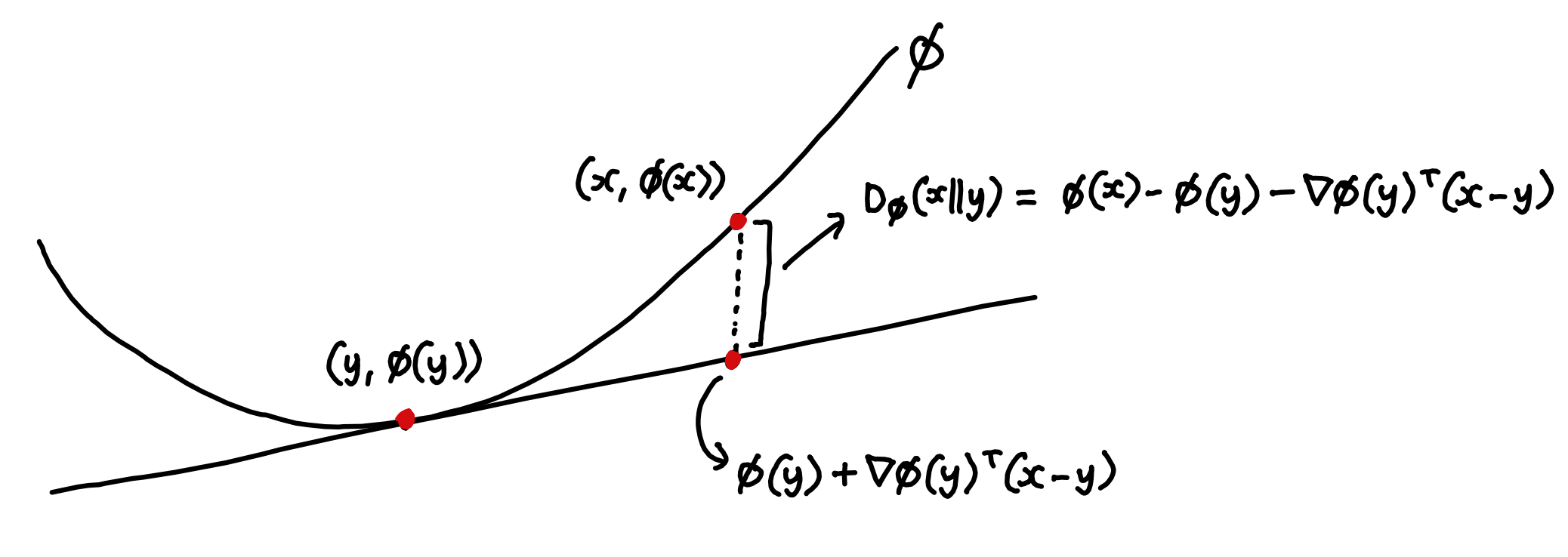
It turns out that there's a natural way to associate any convex function $\varphi$ with a measure of divergence. Since tangents to convex functions always lie below them, we can define Bregman divergence $D_{\varphi }\left(x||y\right)$ as the amount by which $\varphi \left(x\right)$ is greater than the estimate for it you would get by fitting a tangent line to $\varphi$ at $y$ and using it to linearly extrapolate to $x$ .

To do some quick sanity checks for Bregman divergence - if your convex function is the $l_2$ norm squared, then the divergence measure you get is just the squared $l_2$ norm of the vector between your points:

$$D_{||\cdot |{|}_2^2}\left(x||y\right)=||x|{|}^2-||y|{|}^2-2y^T(x-y)=||x-y|{|}^2$$

This is basically what you'd expect - it shows you that when the $l_2$ norm is the natural way to measure how far away something is from zero (i.e. how large it is), then the $l_2$ norm of the vector between two points is the natural way to measure how far one point is from another.

Now, lets go back to the case of probability distributions. Is there any convex function which measures, in some sense, how far away a probability distribution is from zero? Well, one thing that seems natural is to say that "zero" is any probability distribution where the outcome is certain - in other words, zero entropy. And it turns out entropy is concave, so if we just take the negative of entropy then we get a convex function. Slap that into the formula for Bregman divergence and we get:

$$\begin{array}{cc}{D}_{-H}(P\parallel Q)& =-H\left(P\right)+H\left(Q\right)+⟨\nabla H\left(Q\right),P-Q⟩\\ & =\sum _x{p}_x\ln p_x-q_x\ln q_x-\frac{\partial }{\partial q_x}\left(q_x\ln q_x\right)(p_x-q_x)\\ & =\sum _x{p}_x\ln p_x-q_x\ln q_x-(1+\ln q_x)(p_x-q_x)\\ & =\sum _x{p}_x(\ln p_x-\ln q_x)\\ & =D_{KL}(P\parallel Q)\end{array}$$

There's no lightning-bolt moment of illumination from this framing. But it's still interesting, because it shows that different ways of measuring the divergence between two points can be more natural than others, depending on the space that we're working in, and what it represents. Euclidean distance between two points is natural in probability space, when zero is just another point in that space. But when working on the probability simplex, with entropy being our chosen way to measure a probability distribution's "difference from zero", we find that $D_{KL}$ is in some sense the most natural choice.

Final Thoughts

Recapping these, we find that $D_{KL}\left(P||Q\right)$ being large indicates:

1. Your model $Q$ will be very surprised by reality $P$
2. You expect to get a lot of evidence in favour of hypothesis $P$ over $Q$ , if $P$ is true
3. $Q$ is a poor model for observed data $P$
4. You would be wasting a lot of message content if you tried to encode $P$ optimally while falsely thinking the distribution was $Q$
5. You can make a lot of money in betting games where other people have false beliefs $Q$ , but you know the true probabilities $P$
6. (this one doesn't have as simple a one-sentence summary!)

Although (4) might be the most mathematically elegant, I think (1) cuts closest to a true intuition for $D$ .

To summarise what all of these framings have in common:

$D\left(P||Q\right)=$ measure of how much our model $Q$ differs from the true distribution $P$ . In other words, we care about how much $P$ and $Q$ differ from each other in the world where P is true, which explains why KL-div is not symmetric.

To put this last point another way, $D\left(P||Q\right)$ "doesn't care" when $q_x\gg p_x$ (assuming both probabilities are small), because even though our model is wrong, reality doesn't frequently show us situations in which our model fails to match reality. But if $p_x\gg q_x$ then the outcome $x$ will occur more frequently than we expect, consistently surprising our model and thereby demonstrating the model's inadequacy.

---

1. ^{^} Note that the latter case might imply the former case, e.g. if $1\approx q_x\gg p_x\approx 0$ then we are actually also in the former case, since $p_{\neg x}\gg q_{\neg x}\approx 0$ . But this doesn't always happen; it is possible to have asymmetry here. For instance, if P = (0.1, 0.9) and Q = (0.01, 0.99), then we are in the former case but not the latter. If $P$ is true, then 10% of the time model $Q$ is extremely surprised, because an event happens that it ascribes probability 1% to - which is why $D_{KL}\left(P||Q\right)$ is very large. But if $Q$ is true, reality presents model $P$ with no surprises as large as this - hence $D_{KL}\left(Q||P\right)$ is not as large.
2. ^{^} The scalar multiple part is because we're working with natural log, rather than base 2.
3. ^{^} Specifically, the optimal decodable code - in other words, your set of codewords needs to have the property that you could string together any combination of them and it's possible to decipher which codewords you used. For instance, (0, 10, 11) has this property, but (0, 10, 01) doesn't, because the string 010 could have been produced from 0 + 10 or 01 + 0.
4. ^{^} One way you could argue that a distance measure should have this property is to observe that the former two distributions have much lower variance than the latter two. So if you observe a distribution which is either $p=0$ or $p=0.2$ , you should expect it to take much less time to tell which of the two distributions you're looking at than if you were trying to distinguish between $p=0.4$ and $p=0.6$ .